Neural networks models are a flexible class of machine learning algorithms which can be used for both supervised as well as unsupervised learning and can approximate discrete or continuous functions.  They are loosely modeled on the functions of human brains and attempt to allow computers to learn in manner similar to humans.

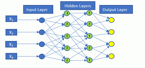
The simplest neural network structure is a single layer feed-forward neural network (or a perceptron) and consists of an input layer, a hidden layer and an output layer as shown in Figure 5.

• The input layer contains the input data which enters the model. These are the independent variables
• The hidden layer in multilayer networks is where the activation functions are applied. Note: neural networks can have many hidden layers. The diagram below displays only two layers. Deep neural networks can contain many hidden layers.
• The output layer produces the output. The output can be binary, categorical or continuous.

Figure 8. Graphical illustration of an Artificial Neural Networks

The following is a quick and dirty explanation of how the neural network trains the data. First, each connection to a hidden or output node has an assigned weight. The node then applies an activation function to the sum of these weighted inputs and generates an output. The output values are then compared to the actual values to calculate an error rate or cost function (there are many types of cost functions). The information is then fed back into the neural network to update the weights by a process known as back-propagation.  This process is repeated until the error rate or cost function is minimized.

Artificial Neural Networks, Convolutional Neural Networks, Recurring Neural Networks and Reinforcement Learning (all of which fall under Deep Learning) are basically extensions of the neural networks theory notably.

Disadvantages:

• Neural Networks are prone to over-fitting.
• While Neural Networks are flexible the learning curve is also steeper than many of the other algorithms. The responsibility for calibrating the model largely lies with the user. Decisions must be made as the number of hidden neurons, the maximum steps for the training of the neural network must be set large enough to ensure convergence, what activation function to use, number of iteration, etc.
• The training time for neural networks in usually longer than other algorithms described previously in the blog.

Figure 9 displays the conditional matrices derived by the Neural Networks approach. It displays the forecasted migration matrices conditioned on Baseline, Adverse, and Severely Adverse economic conditions.

library("RTransProb")

for (i in c(24,25,26)) {
  tic()
  data <- data

  histData <- histData.normz

  predData_ann2 <- predData_ann
  predData_ann2 <- subset(
    predData_ann2,
    X == i,
    select = c(Market.Volatility.Index..Level..normz

    )
  )

  indVars   = c("Market.Volatility.Index..Level..normz"

  )

  startDate = "1991-08-16"
  endDate   = "2007-08-16"

  depVar <- c("end_rating")
  pct <- 1
  wgt <-  "mCount"
  ratingCat <- c("A", "B", "C", "D", "E", "F", "G")
  defind    <- "G"
  ratingCat <- as.numeric(factor(
    ratingCat,
  levels = c('A', 'B', 'C', 'D', 'E', 'F', 'G'),
  labels = c(1, 2, 3, 4, 5, 6, 7)
  ))
  defind <- as.numeric(factor(
    defind,
    levels = c('A', 'B', 'C', 'D', 'E', 'F', 'G'),
    labels = c(1, 2, 3, 4, 5, 6, 7)
  ))

  method    = "cohort"
  snapshots = 1
  interval  = 1
  hiddenlayers = c(1)
  activation = "logistic"
  stepMax = 1e9                #increase to make sure the DNN converges
  calibration = "FALSE"
  rept = 1

  ann_TM <-
    transForecast_ann(
      data, histData, predData_ann2, startDate, endDate, method, interval,
      snapshots, defind, depVar, indVars, ratingCat, pct, hiddenlayers,
      activation, stepMax, rept, calibration
    )
  print(ann_TM)

  toc()
}

Continue Reading

Previous: Machine Learning and Credit Risk (part 4) – Support vector Machines

Next: Machine Learning and Credit Risk (part 6) – Multi-class Linear Discriminate Analysis